Maximum value rolled on a handful of dice

Suppose you roll 2D6. Instead of adding the results together, you take the maximum of both dice. What would be the corresponding probability distribution?

(We will note the result of such a roll as max(2*D6) – to make distinction with the commonly used notation 2D6 which means adding the values.)

It’s of course intuitive to see that the probability of getting a result of 6 using such a roll would be higher compared to simply rolling a single D6. After all, there’s a higher probability of one of the dice scoring a 6. Likewise, the probability of rolling a 1 would be smaller, since this would require both dice rolling a 1, and this is only a 1/36 event compared to a 1/6 event when rolling a single die.

But what are the probabilities exactly?

As you can often do when computing probabilities for a low number of total outcomes, we can simply list all possible outcomes, and add up the probabilities for all relevant outcomes we wish to consider. The table below lists all possible combinations of rolling two ordinary D6, with the maximum value of both dice listed. We have highlighted all results that produce a maximum rolled value of 4.

max(2*D6)	1	2	3	4	5	6
1	1	2	3	4	5	6
2	2	2	3	4	5	6
3	3	3	3	4	5	6
4	4	4	4	4	5	6
5	5	5	5	5	5	6
6	6	6	6	6	6	6

Each cell in the table has a probability of 1/36, so if we add everything together, we have the following overall probability table for max(2*D6):

Result of max(2*D6)	probability
1	1/36 = 2.78%
2	3/36 = 8.33%
3	5/36 = 13.89%
4	7/36 = 19.44%
5	9/36 = 25%
6	11/36 = 30.56%

A first thing you can see is that the probabilities are not evenly distributed, as expected. On closer inspection, the probabilities go up in a linear trend: each results shows an increase of 2/36 = 5.56% over the previous one.

This also becomes obvious when we plot the values in a graph (all graphs in this blogpost are made using the online tool anydice.com).

A similar reasoning can be made for plotting the probability outcomes of the minimum of 2 dice. The graph below shows both max(2*D6) and min(2*D6).

And of course, varying the die type doesn’t make much of a difference for our analysis. The graph below shows plots for the maximum of 2 dice, for the usual type of dice used in games.

What about the maximum of rolling 5 D10’s?

So what if we roll more dice? Again, when rolling more and more D6’s, you would expect higher and higher probabilities of rolling a 6 as the maximum value. To compute these probablities exactly, let’s look at the table more carefully.

To count all cells with a result equal to 4, we can also count all cells with a result equal to or less than 4 (green and orange cells), and subtract the cells with a result equal to or less than 3 (green cells only). This leaves us with the number of cells that have a value exactly equal to 4 (orange cells).

Max(2*D6)	1	2	3	4	5	6
1	1	2	3	4	5	6
2	2	2	3	4	5	6
3	3	3	3	4	5	6
4	4	4	4	4	5	6
5	5	5	5	5	5	6
6	6	6	6	6	6	6

 As you can see, the green cells (result equal to or less than 3) form a  square, and the number of green cells can be expressed as the square of 3 or 3*3 = 9. Likewise, the number of cells with a result equal to or less than 4 add up to 4*4 = 16. Thus, the number orange cells (result equal to 4) equals 16 – 9 = 7. Dividing 7 by 36 (the total number of possible outcomes) gives us the desired probability 7/36.

In general, we can compute the probability of max(2*D6) being equal to x as:

Prob(x) = (x*x – (x-1)*(x-1)) / 36

We can generalize this to a higher number of dice. If we would roll 3 dice, the above square becomes a “cube” in the (3-dimensional) table, and we count the number of cells as x*x*x. For n dice, we go to an n-dimensional space, and we can write:

Prob(x) = (xⁿ – (x-1)ⁿ)/6ⁿ

If we want to roll a Dy with y faces instead of an ordinary D6, the formula becomes:

Prob(x) = (xⁿ – (x-1)ⁿ)/yⁿ

The graphs below show the resulting probabilities for rolling an increasing number of D10, and each time taking the maximum value as the result.

 The probabilities of rolling higher numbers go upward as you roll a higher number of dice, as can be expected.

Cumulative probabilities

In a recently published fantasy ruleset (Oathmark, Osprey Games), there is a mechanism in which you roll max(2*D10), and you need to roll equal or higher than a target number to activate a unit. Thus, we are interested in the cumulative probability: what is the probability of rolling *at least* a given value.

For this, we need to sum all probabilities for that target number or higher. The resulting graphs, again for an increasing number of D10, are shown below.

One can wonder whether this specific mechanic is worth it. Does rolling max(2*D10) really make a difference compared to some other – mechanically more familiar or simple die rolls?

The graph belows shows the cumulative plot (rolling equal or higher than a target number …) for max(2*D10), tha familiar 2D6, and D8+3.

As you can see, the differences are negligible, especially if you look in the range 5 to 10, which is the interesting range for activation target numbers.

Conclusion

Personally, I don’t really like the highest-roll-mechanic. It requires rolling multiple dice (and using only 1 as the final result), and it can easily be replaced by a more familiar die roll.

1 hit for 10 damage, or 10 hits for 1 damage each?

Many wargames have a mechanic that requires a number of damage points to be inflicted for a target to be eliminated. Damage is usually caused by a number of shots, each shot having a certain probability of hitting the target, and each shot causing a number of damage points. Thus, we already have various variables with which we can shape our mechanic: the number of total damage points needed to kill the target; the probability of each shot causing a hit; and the number of damage points per successful hit. Given these variables, it is quite naturally to ask how long it will take before the target is eliminated. And is it better to have a mechanic in which we need 10 hits, causing 1 damage each, or needing one mega-hit causing 10 damage by iself?

2 cruisers closing in on a battleship ...

Do we prefer many shots, many of them on target, but each doing a tiny amount of damage?

... or do we rather prefer many shots missing, but the one shot that hits, causing the ship to sink?

 Mathematics

To get a good insight in the mechanic, let's take a look at the math. First, let us define some of the parameters:

• p_success: the probability (a number between 0 and 1) with which a shot hits the target. Let's assume p_success is the same for all shots.Translated into a die roll, a D6 that requires 5+ to hit has p_success = 0.33, a D10 that requires 4+ to hit sets p_success equal to 0.6, and so on.
• s: the number of successful shots needed to kill the target. Again, to keep things simple, let's assume that all hits cause the same amount of damage d. Thus, if the target has D damage points, s = D/d (rounded up). E.g., if a successful shot causes 3 damage, and we shoot at a 10-damage target, we need 4 successful shots (10/3, rounded up) to kill the target.
• n: the total number of shots (trials), included misses. Not every shot will hit the target, as is obvious from p_success. n will always greater or equal than s. If we are lucky, we can kill the target with s number of shots, but the lower the value of p_success, the more shots we will need to reach s successful shots.

So, we can phrase the mathematical problem as follows: what's the probability of s hits occurring in a sequence of n shots, with the last shot being successful (and thus killing the target)? Or to put it differently: what is the probability we will need n shots, given s successful shots with the n-th shot being the last successful s-th shot?

This problem might look familiar to another problem we have analyzed before, the Buckets of Dice procedure. When rolling  n dice, we are often interested in how many dice will score a success given a certain probability of success for each dice. The binomial distribution expresses the probability that we score s successes, given n dice. But now, we want something slightly different. Instead of fixing the number of trials n, and keeping the number of successes as a changing variable, we now want to fix the required number of successes s, and consider the total number of trials n as a variable. It is a minor change of viewpoint, but we can still use the same mathematical framework.

Before we can write down the equations, we need some additional insights:

• The first insight we need is that it doesn't matter which of our shots are successful, except for the last one. If we want to reach 4 successful hits in 10 trials, we know that the 10th shot needs to be a success (the 4th hit), but the previous 3 hits can happen anywhere in the previous sequence of 9 shots.
• The second insight is that if 3 shots can happen anywhere in a sequence of 9 shots, the mathematics don't care whether those shots are taken in sequence or all together, as long as all shots are independent from each other. Thus, we can use the binomial distribution as described by the Buckets of Dice method to describe the probability distribution of s-1 shots being succcessful, out of n-1 total number of shots. Using the same notation as in our Buckets of Dice blogpost, we can write this distribution as Bin(s-1, n-1, p_success).

Now we need to combine both observations. The first s-1 succesful hits can happen anywhere within the first n-1 shots. The n-th shot must be the s-th succesful hit, and this shot will be succesful with a probability equal to p_success. Thus, the complete probability distribution for s succesful hits, using n shots, with the last being a success, can be written as:

NBin(s, n , p_success) = Bin(s-1, n-1, p_success) * p_success 

Such a distribution is known in mathematics as a Negative Binomial Distribution, hence the notation Nbin (see also the appendix for some more information).

The relationship with the more well-known Binomial Distribution is clear, but as mentioned before, the viewpoint is slightly different. The Binomial Distribution is mostly concerned with the probability of scoring k successes out of n trials; the Negative Binomial distribition is interested in the probability of needing n trials to score s successes.

Analysis

So, what does this distribution look like? Many spreadsheet programs have the Negative Binomial Distribution built in, but you can also use the above formulation, expressing it as the product of the Binomial Distribution (which also often is a pre-defined function in many spreadsheet programs) multiplied by the probability p_success.

Let's look at some simple cases first, just to get a feeling of how this function evolves with various parameter settings.

Let's first set p_success = 2/6, which means rolling 5 or 6 on a D6 in order to score a hit. Let us further assume we want to score 2 successful hits. The graph below shows the probability of number of total shots n needed.

As you can see, there is zero probability n equals 1 (obviously, since we need 2 successes), and n = 3 or n = 4 is the most likely outcome, each with roughly 15% chance of occuring. The probability we will need more than 4 trials decreases gradually.

Let us now assume we set p_success = 1/6, in other words, a successful hit will on average only happen once every 6 shots. The resulting distribution for the total number of shots n needed is shown below.

You can immediately see the most likely outcomes are n = 5 to 8, and again there is a decreasing probability we will need ever more shots, although the decrease is not as sudden as with p_success = 2/6.

Now let's very the number of required successful shots, while keeping p_success at 2/6. The graph below shows the probability distribution.

Since we need a higher number of successes, the graph shifts to right, in this case with a most likely outcome for n = 9 or 10, again with a gentle decrease for higher numbers of n.

I guess you are curious for other values of p_success and s as well, so here are the complete graphs. First, the probabilty disctributions for different values of p_success, fixing the number of successes on 2.

And here a variable number of successes, with fixing the probability for scoring a succesful hit:

Note the atypical shape of the distribution for 1 success, which is to be expected, since exactly the last shot needs to be a success, and all previous shots need to be misses.

Expected value for n

The above graphs might give you some insight in the mathematics, but how can we translate this into useful gaming mechanics? The first thing a game designer might be interested in, is the expected value of the total number of shots n (successes and misses), in function of p_success and s.

We will not go through the mathematical derivation, but the expected value for n (the expected value E(n) is the average value for n  if we would conduct or procedure an infinite number of times), equals s / p_success.

This is not so surprising, if we fill out some numbers:

• If p_success = 1/6, and s = 1 (we need one successful shot, we a chance of 1/6 of scoring one), we can expect to need 6 shots.
• If p_success = 3/6, and s = 2, then E(n) = 2*6/3 = 4, which means we can expect to need 4 shots in order to score to 2 successful hits with a success ratio of 50%.

So, what does this formula teach us?

• doubling the value of s, while keeping p_success a constant, will double the value of E(n). Or more generally, increasing or decreasing the value of s by a certain ratio, will also multiply E(n) by that same ratio.
• doubling the value of p_success, while keeping s a constant, will halve the value of E(n). Or more generally, increasing or decreasing p_success by a certain ratio, will inversely proportional change the value of E(n).

If we know put some more gaming terms into our equation, and if we want to keep the initial example of having to score a number of hits D on a target, with each hit inflicting d damage points, we can say that s = D/d. But since E(n) = s / p_success, we can now say that:

E(n) = D / (p_success * d)

Thus, we have the expected number of shots (which can translate in a number of turns in the game), the total amount of damage needed, the chance for scoring a hit, and the damage per hit, in one nice formula. You can play around with the values, keeping some fixed while changing others, and see what the outcome is.

Standard deviation
The standard deviation of a stochastic process is a measure for how far any given experiment can deviate from the expected value. After all, the expected value is only an average number, but any single experiment can produce a number lower or higher than the expected value.

The standard deviation for n, is given by the square root of (1 - p_success) * s / (p_success * p_success). This seems like a rather convoluted formula, and you might want to plug in some numbers to see how the standard deviation will change with various parameters, but you can see that the standard deviation:

• ... increases proportional to the square root of s  if p_success is kept constant. Thus, quadrupling s, will only double the standard deviation.
• ... decreases with higher values of p_success, due to p_success in the denominator. Roughly we can say that the standard deviation changes inversely proportional to p_success.

A full analysis would lead us to far, but again you can try out some numbers yourself. One last thing to note is that you can also compute the relative value of the standard deviation vs E(n). This turns out to sqrt ((1-p_success)/s). Thus, increasing the number or s, while keeping p_success a constant, will make the relative spread narrower around E(n).

Gaming mechanics

What does this all mean for gaming mechanics?

We know that E(n) = D / (p_success * d). Now suppose we want to find values for the different parameters, but keeping the expected value E(n), which can act as a proxy for the number of turns needed to sink a target, the same. Also suppose we keep D a constant (after all, D the total number of damage points, and is in some sense an arbitrary number). For 2 different gaming mechanics, each with different values for d and p_success, and forcing E(n) to remain a constant, we can then say:

p_success_1 * d_1 = p_success_2 * d_2

Thus, the damage points per successful shot should scale inversely proportional to the probability of a successful shot. If we set p_success_1 = 2/6, and d_1 = 6 points, then this is equivalent to setting p_success = 4/6, and d_2 = 3 points.

When we say both procedures are equivalent, they are both equivalent in E(n), the expected number of shots needed to sink the target. But there will be a difference in the standard deviation. However, to compute the standard deviation, we need to set a value for s. s is determined by D and d, since s = D/d. So, the standard deviation, equalling sqrt((1-p_success)*s/p_success*p_success) is now rewritten as sqrt((1-p_success)*D/p_success*p_success*d).

So, let's plug in some numbers, and let's set D at 12:

• p_success = 1/6, d = 12 => s = 1, E(n) = 6, stdev = 5.47
• p_success = 2/6, d = 6 => s = 2, E(n) = 6, stdev = 3.46
• p_success = 4/6, d = 3 => s = 4, E(n) = 6, stdev = 1.73

The graph for these 3 settings is shown below.

Playing around with the numbers is of course fun, but there are others things to consider. E.g. setting d = D (i.e. a single shot kills the target), means avoiding bookkeeping (tracking the number of hits, damage points left, ...). Setting d different from D implies keeping track of the amount of damage inflicted. Whether or not that's a good thing, depends on other mechanisms in the rules.

Conclusion

Whether you want one big shoot that kills in an instant, or a sequence of low intensity shots that require many turns to kill, keep in mind that what really matters is the expected number of shots (misses and hits) needed, as well as the standard deviation on that number.

Appendix:

1. The Negative Binomial Distribution is described in various ways in different textbooks. Often, it is defined as a fixed number of failures in a sequence of trials, thereby reversing the definition of success and failure as we have used in this blogpost. Sometimes, instead of the total number trials n, the number of failures and number of successes are used as parameters, wit n being the sum of the two. But it all ends up describing the same type of distribution. For more information, see https://en.wikipedia.org/wiki/Negative_binomial_distribution

It has been a while (again)

It has been a while since I posted something on this blog, but job and personal issues have kept me from doing so. However, I have full intentions of returning my attention to this blog once the exam period at my university is over and the summer monts begin ...

Hidden troop movement

On a real battlefield, not everyone can see everyone else all the time. Troops might be hidden from the enemy, laying in ambush, seeking cover behind a hill, etc. This is especially true for the modern "empty battlefield", which doesn't have the colourful uniformed regiments marching in very visible formations across the field of fire towards the enemy.

Dealing with hidden troops (and hidden movement) on the gaming table has always been a challenge for the wargamer. In essence, there's no good solution to it, because the knowledge of the wargamer is not the same as the knowledge of the troops or the commanding general on the table. Dealing with hidden troops in wargaming is one of those issues that touch on the problem of the all-seeing gamer, and hence, any mechanic will always be a workable compromise.

Some mechanics might work better in some setups, because we need to distuinguish between different situations:

• Is there an umpire present who can act as a keeper of "unknown" information?
• Is only one side using hidden troops? The classic example is an attack./defence scenario, in which the defender is (initially) hidden, or an ambush scenario, where the ambushing troops are hidden. 
• Are hidden troops static (e.g. the defensive side in a scenario), or can hidden troops move across the table and still remain hidden?
• Can troops become hidden again after having become exposed?
• Is the location of hidden troops known to the player controlling these troops?
• ...

Each of these situations might favour a particular mechanic over another.

This post will zoom in on a few mechanics I have used in the past to represent hidden troops on the table. Note that I'm only discussing the hidden *location* of troops on the table, not the nature or characteristics of troops which might also be unknown to one or both players. Neither will I deal with movement that is unknown even to the controlling player (e.g. troops getting lost in a forest). Perhaps these might be the subject of a future post.

Using a map of the gaming table

Especially older wargaming publications promote the idea of using a map of the gaming table to track the position of troops. After each movement phase, an umpire should check the maps of both players and determine whether any troops become visible to the other player. Those units are then put on the table. Easy enough, but it only really works when an umpire is available.

The idea goes back to the original 19th century Kriegsspiel, in which there were 3 tables: one for each side, and one for the umpire. Only the umpire's table has all the information, and both sides gradually discover the location of the enemy troops. The use of three separate tables is not really a viable possiblity for many wargamers (except perhaps in a well-planned-in-advance club game), but the use of a separate smaller map is a possibility, as long as an umpire is present.

One instance in which we have used maps frequently is in attack/defence scenarios. The defender deploys hidden (using a map), and all attacking units are on the table. Once the (static) defending units become visible to the attacker, they are deployed on the table, and cannot become hidden again. No umpire is needed, and it is a simple mechanic to keep the attacker on his toes during the initial movement phases of the scenario.

Waypoints

Instead of dealing with maps, the location of hidden troops can be recorded by using easy-recognize features on the gaming table. E.g. one might make a note on the troop roster, stating something like "at the end of the road" or "in the little wood near the village".

Once a waypoint becomes visible for an enemy unit, any unit at the waypoint is placed on the gaming table. This approach works well if only one side is hidden, since if both sides would use waypoints, an umpire is still needed to cross-check hidden locations and decide who has become visible for whom.

To facilitate the use of way-points, I use small numbered markers on the battlefield. Instead of writing down things such as "the edge of the wood", or "behind the hill", a reference to a numbered marker is much easier. If you place enough of these numbered markers on "sensible" locations of the battlefield, most locations can be specified rather easily.

I use a set of small pebbles on which I have inked numbers 1-20, so they can blend in nicely with the scenery.

Dummy units

A total different approach for handling hidden troops on the gaming table, is to use dummy units. Dummy units are acting as a "placeholder" for real units, or perhaps there's no unit at all! In a sense, the location of troops becomes hidden by adding false information on the battlefield. The opponent can see the dummy units, but he doesn't know what dummy units are real and which are false. Hence, the location of the real units is effectively hidden.

The player controlling the dummy units should of course be aware which ones are "real", and he should keep track of that as well.

For some of my skirmish games, I use cheap black-painted, grey-drybrushed figures to indicate dummy units. As soon as contact is made with such a dummy unit, it is replaced by properly painted figures. Numbered labels attached underneath the base of the dummies allows for the controlling player to identify which units are which.

Dummy units: black painted, grey drybrushed figures.

This mechanic does not require waypoints as described above, but it does require some more figures (or other markers) to use as dummies. Moreover, the use of dummies adds a new dynamic to the game. The enemy can see where all the units are moving to, but can never be sure whether a concentration of dummies is real, or is only a ruse. It is also possible for both sides to use dummy units, hence avoiding the need for an umpire.

It's been a while ...

It has been a while since I posted something new on this blog. But there's good news, I have 3 posts in the making:

• One about the mathematics of doing a single 10-damage hit, or doing 10 1-damage hits;
• One about mechanics for using hidden troops on the table;
• One about further limitations of grids, and more specifically, hexagonal grids, which is inspired by an image in Phil Sabin's book "Simulating War", and which is shown below. Can you spot the problem?

Putting units or actions in the outer loop ...

Many of the discussions regarding rules design in miniature wargaming involve the turn sequence, and how to structure it in order to achieve some desired effects. Over the years, there have been many different variants of the turn sequence, illustrating various schools of thoughts on how to organize the game. Often, discussions are framed as IGO-UGO vs unit-activation, but the spectrum is more varied than that. See also my earlier post on discussing various ways of looking at the turn sequence.

In this post, I will offer a slightly different way of looking at the turn sequence, and how it can affect rules design.

Action-based turn sequences

In an action-based turn sequence, the turn is defined as a (strict) sequence of actions, and within each action, every units can do exactly that action. This is best illustrated with the classic move-shoot-melee-morale sequence. First, we have the movement phase, in which all units get to move. Then we have the shooting phase, in which all units can shoot. The same goes for the melee phase and the morale phase.

In computer programming terminology, one can see such a turn sequence as 2 nested loops . An outer loop loops over all actions, and an inner loop, for each action, loops over all units doing that action:

• for each action X (in fixed order move, shoot, melee, morale):
• for each eligible unit Y (order usually chosen by player):
• unit Y does action X

Such a turn sequence has a number of advantages - there is a fixed order for all actions, and this implies one can be sure that all movement has happened before shooting and melee, morale checks are performed after all combat etc. This can lead to a design in which those various phases of the turn are strongly coupled. However, it also often leads to rules in which all turn phases use separate mechanisms which have not much in common from a procedural point-of-view. The mechanisms for shooting and melee can be very different, and morale usually is a separate subsystem.

An important and crucial disadvantage is that actions which are not explicitly listed in the turn sequence cannot be added to the games engine in an elegant manner. Such actions are often defined in terms of an existing action. E.g. setting a building on fire might take half a move; or instead of fighting a unit might build (part of) a bridge. An alternative solution is to add such additional actions explicitly to the turn sequence. E.g. one can imagine having a separate "engineering phase", or "spell casting phase". The drawback is that such specialized actions become very visible in the outer loop, while relatively few units might be eligible to act on them. These actions might also be rarely used during the entire game, depending on the specific scenario. In a fantasy ruleset we used during the late 90s, there was a phase in the turn sequence called "Morph Friendly Cyclics". It always gave rise to the same joke in each and every game. "Hold on guys, we forgot the Morph Friendly Cyclics phase! Friendly cyclics anywhere? No friendly cyclics? Are you sure? Ok, now we can move on ... "

Unit-based turn sequences

In computer programming, 2 nested loops can often be interchanged. We can also do this in the turn sequence. Instead of defining the turn as a loop over all actions, we define it as a loop over all units:

• for each unit Y (order usually chosen by player, and/or driven by an activation mechanism):
• for each eligible action X (chosen from a list of possible actions):
• unit Y does action X

Such turn sequences are often called unit-based activation, since the units might be activated by die rolls, cards in hand etc. There might even be a terminating condition (e.g. a failed die roll), indicating the end of the turn. When a unit is activated, there usually is a choice of what actions, or a combination of actions (perhaps expending a budget of 'action points'), can be executed with that unit.

The main disadvantage of such a sequence is that it is difficult to maintain coherency between units. E.g. if one would like to maintain a battle line, and one cannot be sure that all units can move forward during this turn (e.g. if there is a possibility not all units might get activated), this can really frustrate player or result in ahistorical behaviour of the troops on the gaming table. Often, a mechanism for activating a group of units is necessary as part of the activation procedure.

On the other hand, there is a big advantage when one wants to add additional types of actions. Since actions do not drive the turn sequence at the top-level, adding actions does not change the turn structure. Rather, actions are an add-on to an already existing structure, which makes it easier to maintain coherent procedures and game mechanisms.

This does not prevent from actions having their own disparate procedures, but it does create a structure in which a coherent mechanism for resolving actions is more viable. One of the best examples is the Basic Roleplaying System by Chaosium. It exists in many different variations (the Call of Cthulhu rulesystem probably is the best-known). Looping over the characters is the outer loop (as in most roleplaying games), and each action - whether it is searching in a library or swimming across a pond - is resolved by checking a D100 vs a target number. That results in a very elegant and tight design, and adding new types of actions is rather straightforward.

The same structure can be used in miniature wargaming. Whether you want to add engineering actions, special movement or shooting actions, or actions invented for a specific scenario only, they can be fitted much easier in the overall game structure as opposed to an action-based turn sequence.

Triangular Grids

I am a fan of using grids for miniature wargaming. My wargaming table has a permanent Hexon terrain system laid out, but I've also played games on a rectangular grid, most notably my Flagstone Fleets game. See also the Table of Contents for previous discussions about grids.

In this blogpost, I would like to discuss the triangular grid. I think it's a grid that has not been fully explored in wargaming (hexagonal grids and square grids are getting much more attention), but it is worthwhile to look at some of its advantages and disadvantages.

Relation between the triangular and hexagonal grid

There is a strong relation between the classic hexagonal tiling, and a triangular tiling.

Mathematically, they are each other's dual tiling. This means that if you take the centre points of each hexagon, and you connect these centre points together, you get the triangular tiling. This also works in the other direction: if you take the centre points of each triangle, and connecting them together, you get the hexagonal tiling.

This duality results in a nice property: when playing a game on a triangular grid: placing the pieces on the corner points and moving them along edges, is equivalent to playing that game on a hexagonal grid by placing the pieces inside the hexagons and moving them across edges. And vice versa, playing a game on the corners and along edges of a hexagonal grid, is equivalent to putting the pieces in the triangles and moving them across edge boundaries.

There is however a major issue with the triangular grid, which is the asymmetry of connections between the triangles. Unlike a hexagon grid, triangle can connect edge-to-edge, but also point-to-point in various configurations. THis is also the case in a square grid, but in a triangular grid there are different ways in which triangles can connect point-to-point. This lack of symmetry is the most likely reason why triangular tiles have not been really considered for wargaming.

Has the triangular grid been used before?

When trying to look up whether (board) wargames make use of a triangular grid, surprisingly few results turn up. Most of the games that use a triangular grid, use the dual property, effectively using a hexagonal grid. The triangular grid is then merely an esthetic element in the design of the game. See e.g. games that employ the "Triangle System", See also this page at Forsage Games.

Most games that use the triangles themselves as areas usually are abstract boardgames. Some examples are: Blokus Trigon or Go played on a triangular grid.

Counting distances

Let us assume we do want to design a miniature wargame using a triangular grid. One of the things we need is a counting procedure for counting distances from one grid cell to another cell, and preferably, we would like that counting procedure to approximate the Euclidean distance between the centre points of both grid cells.

Using some simple goniometry, and setting the distance between the (barycentric) centre points between 2 adjoining triangles to 1, we arrive at the following relations:

Taking the red dot as starting point, we see that we can get to edge-to-edge triangles (yellow dots) using distance 1. The triangle directly opposite (blue dot) requires distance 2. Both triangles that touch the starting triangle, but are not directly opposite (yellow dots), are at a distance equal to the square root of 3, or 1.73.

Rounding up 1.73 to 2, we get the following, rather simple, counting procedure for measuring distances:

• When moving from edge-to-edge, count 1;
• When moving from point-to-point (any configuration), count 2.

This looks like a nice and relatively simple procedure for counting distances. Another way to look at this, is to construct a hexagonal grid on top of the triangular grid, by inscribing each triangle with a hexagon, and putting additional hexagons at the corner points (note that this is a different hexagonal grid as opposed to the dual grid as described above):

(Image from "20 Fun Grid Facts (Hexgrids)")

The yellow and blue triangles (or the yellow and blue hexagons) form our triangular grid. When moving from a yellow to an adjacent blue hexagon (i.e. moving on the triangular grid from a yellow to a blue triangle), you can do that directly, at a cost of 1 movement point. But when you move to a hexagon whose corresponding triangle is touching at a corner, you have to pass through a green corner hexagon, resulting in 2 movement points if you would count along the hexagonal grid. So, our distance rules derived above can also be considered as moving on the underlying hexagonal grid - albeit by disregarding the green hexagons as shown in the diagram above.
(You might wonder how this is possible, given that we have rounded one distance 1.73 to 2 ... but there are also 2 modes of moving on a hexagonal grid: straight ahead from hexagon to hexagon, or in a "zig-zag" pattern, which correspond to our differently connected triangles ... these two movement paths are not exactly equal, although we often consider them as such on the hexagonal grid.)

Ok, let's put it all together. How far can we move on a triangular grid given various amounts of movement points? The diagram below illustrate the movement ranges, using 1 movement point to move across an edge, 2 movement points to move across a corner.

The blue, green and orange triangles indicate the range using 3, 5 and 7 movement points. The dotted black arcs have radius equal to 3, 5 and 7. The dotted red arcs are scaled with a cosine(30 degrees) factor. This allows comparing the "zig-zag" movement when one would move along the horizontal row of adjacent triangles.

Facing, Battlelines and firing arcs

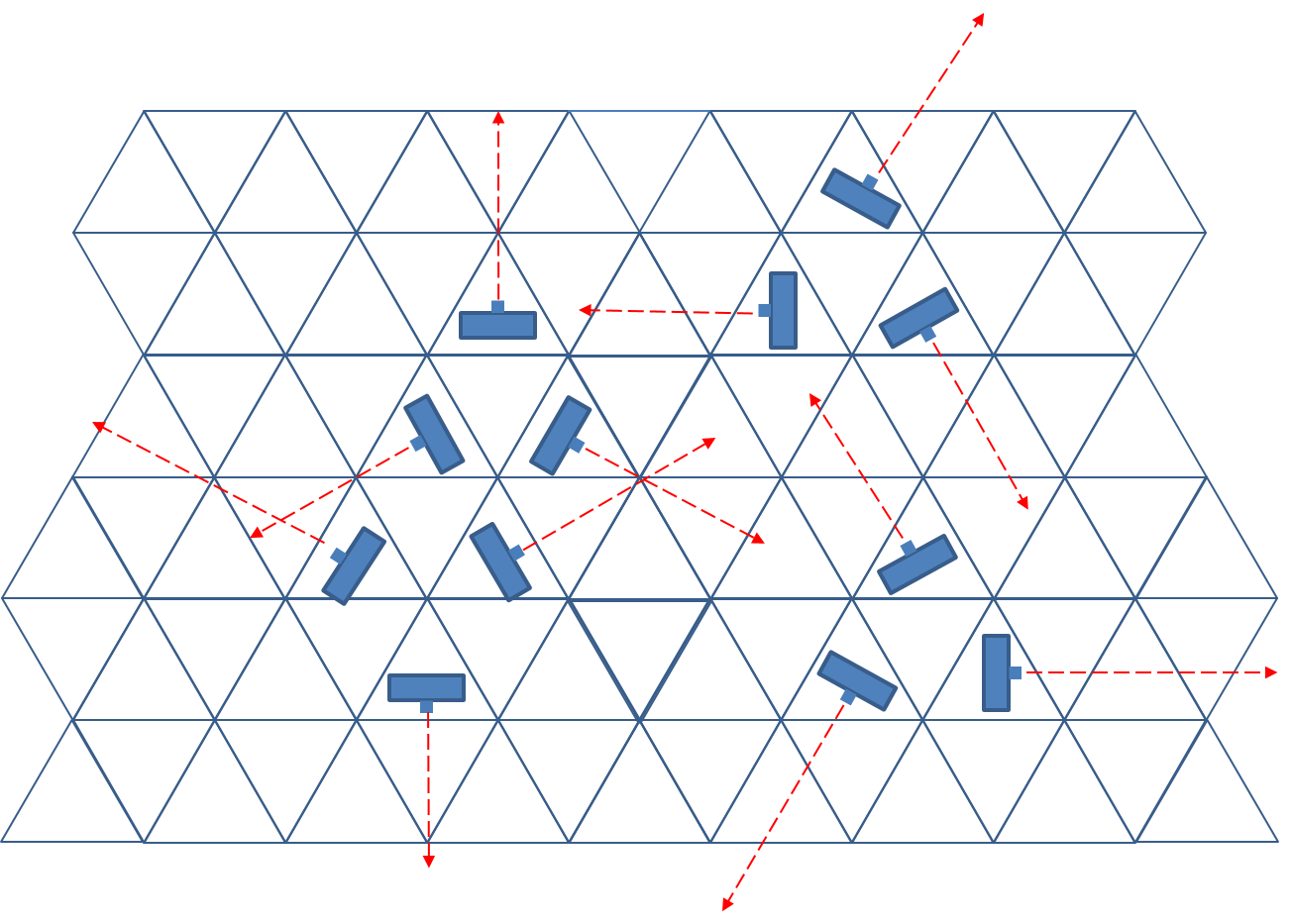
When located in a triangle, a unit can be oriented in 12 different directions: 3 sides, 3 corners, but there also 6 other directions that line up with rows of triangles (see diagram below). This is not unlike a square grid where you have 8 natural facings, or a hexagonal grid that has 12 facings (6 edges + 6 corners).

Square grids have 3 natural main directions along one which can put troops next to each other: vertical, horizontal, and diagonal. A hexagonal grid has 3 main directions, and 3 "zig-zag" directions. What about the triangular grid? The triangular grid also has 6 main directions, as shown below (the 2 other symmetric directions at 30 and 60 degrees are not shown).

The orientation and facings, having 12 "natural" directions on the grid, might be the biggest advantage of the triangular grid. However, just an in squares, the connections between the grid cells is asymmetric. But this is also the case when considering the "zig-zag" directions in a hexagonal grid.

Firing arcs become a little more complex. The diagram below shows firing arcs at 60 degrees, and a distance of 4, using the counting metric as derived above. Note the little discrepancy in the firing arc for the unit on the right.

All this seems workable, but it takes time getting used to.

Conclusion

So, should we use the triangular grid for our miniature wargames? Honestly, I don't know yet. I will have to run a test game or two ... but any other experiences or insights are certainly welcome!